Charge susceptibility, longitudinal magnetic susceptibility and optical conductivity
Correlator of a Hermitian operator \(\hat O\) with itself is defined as
\[\chi(\tau) = \langle\mathbb{T}_\tau \hat O(\tau) \hat O(0)\rangle.\]
Common examples of such correlators are the longitudinal magnetic susceptibility \(\langle\mathbb{T}_\tau \hat S_z(\tau) \hat S_z(0)\rangle\), the charge susceptibility \(\langle\mathbb{T}_\tau \hat N(\tau) \hat N(0)\rangle\) and the optical conductivity \(\langle \mathbb{T}_\tau \hat j(\tau) \hat j(0)\rangle\).
For the Hermitian operators, the auxiliary spectral function \(A(\epsilon) = \Im\chi(\epsilon)/\epsilon\) is non-negative and symmetric.
This kind of correlators is treated by the BosonAutoCorr kernels, which are faster and more robust than BosonCorr.
Perform analytic continuation using the BosonAutoCorr kernel
# Import HDFArchive and some TRIQS modules
from h5 import HDFArchive
from triqs.gf import *
import triqs.utility.mpi as mpi

# Import main SOM class and utility functions
from som import (Som,
                 fill_refreq,
                 compute_tail,
                 reconstruct,
                 estimate_boson_corr_spectrum_norms)

n_w = 501                    # Number of energy slices for the solution
energy_window = (-2.5, 2.5)  # Energy window to search the solution in
tail_max_order = 10          # Maximum tail expansion order to be computed

# Parameters for Som.accumulate()
acc_params = {'energy_window': energy_window}
# Verbosity level
acc_params['verbosity'] = 2
# Number of particular solutions to accumulate
acc_params['l'] = 2000
# Number of global updates
acc_params['f'] = 100
# Number of local updates per global update
acc_params['t'] = 50
# Accumulate histogram of the objective function values
acc_params['make_histograms'] = True
# Right boundary of the histogram, in units of \chi_{min}
acc_params['hist_max'] = 4.0

# Read \chi(i\omega_n) from archive.
# Could be \chi(\tau) or \chi_l as well.
chi_iw = HDFArchive('input.h5', 'r')['chi_iw']

# Set the error bars to a constant (all points of chi_iw are equally important)
error_bars = chi_iw.copy()
error_bars.data[:] = 0.001

# Estimate norms of spectral functions from chi_iw
norms = estimate_boson_corr_spectrum_norms(chi_iw)

# Construct a SOM object
cont = Som(chi_iw, error_bars, kind="BosonAutoCorr", norms=norms)

# Accumulate particular solutions. This may take some time ...
cont.accumulate(**acc_params)

# Construct the final solution as a sum of good particular solutions with
# equal weights. Good particular solutions are those with \chi <= good_d_abs
# and \chi/\chi_{min} <= good_d_rel.
good_chi_abs = 1.0
good_chi_rel = 4.0
cont.compute_final_solution(good_chi_abs=good_chi_abs,
                            good_chi_rel=good_chi_rel,
                            verbosity=1)

# Recover \chi(\omega) on an energy mesh.
# NB: we can use *any* energy window at this point, not necessarily that
# from 'acc_params'.
chi_w = GfReFreq(window=(-2.5, 2.5),
                 n_points=n_w,
                 indices=chi_iw.indices)
fill_refreq(chi_w, cont)

# Do the same, but this time without binning.
chi_w_wo_binning = GfReFreq(window=(-2.5, 2.5),
                            n_points=n_w,
                            indices=chi_iw.indices)
fill_refreq(chi_w_wo_binning, cont, with_binning=False)

# Compute tail coefficients of \chi(\omega)
tail = compute_tail(tail_max_order, cont)

# \chi(i\omega) reconstructed from the solution
chi_rec_iw = chi_iw.copy()
reconstruct(chi_rec_iw, cont)

# On master node, save parameters and results to an archive
if mpi.is_master_node():
    with HDFArchive("results.h5", 'w') as ar:
        ar['acc_params'] = acc_params
        ar['good_chi_abs'] = good_chi_abs
        ar['good_chi_rel'] = good_chi_rel
        ar['chi_iw'] = chi_iw
        ar['chi_rec_iw'] = chi_rec_iw
        ar['chi_w'] = chi_w
        ar['chi_w_wo_binning'] = chi_w_wo_binning
        ar['tail'] = tail
        ar['histograms'] = cont.histograms
Download input file input.h5.
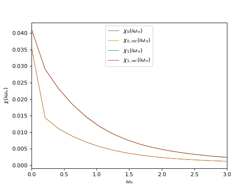
Plot input and reconstructed correlators at Matsubara frequencies
from h5 import HDFArchive
from triqs.gf import *
from matplotlib import pyplot as plt
from triqs.plot.mpl_interface import oplot

# Read data from archive
ar = HDFArchive('results.h5', 'r')

chi_iw = ar['chi_iw']
chi_rec_iw = ar['chi_rec_iw']

# Plot input and reconstructed \chi(i\omega_n)
oplot(chi_iw[0, 0],     mode='R', lw=0.8, label=r"$\chi_0(i\omega_n)$")
oplot(chi_rec_iw[0, 0], mode='R', lw=0.8, label=r"$\chi_{0,rec}(i\omega_n)$")
oplot(chi_iw[1, 1],     mode='R', lw=0.8, label=r"$\chi_1(i\omega_n)$")
oplot(chi_rec_iw[1, 1], mode='R', lw=0.8, label=r"$\chi_{1,rec}(i\omega_n)$")

plt.xlim((0, 3.0))
plt.ylabel(r"$\chi(i\omega_n)$")
plt.legend(loc="upper center")
plt.show()
(Source code, png, hires.png, pdf)
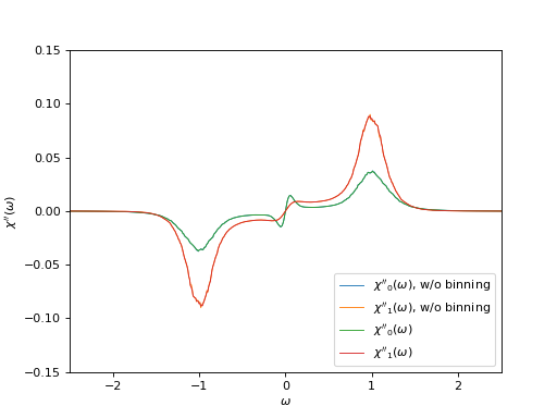
Plot the correlator on the real frequency axis and its tail coefficients
from h5 import HDFArchive
from triqs.gf import *
from matplotlib import pyplot as plt
from triqs.plot.mpl_interface import oplot

# Read data from archive
ar = HDFArchive('results.h5', 'r')

chi_w = ar['chi_w']
chi_w_wob = ar['chi_w_wo_binning']
tail = ar['tail']

# Plot imaginary part of the correlator on the real axis
# with and without binning
oplot(chi_w_wob[0, 0],
      mode='I', lw=0.8, label=r"$\chi''_0(\omega)$, w/o binning")
oplot(chi_w_wob[1, 1],
      mode='I', lw=0.8, label=r"$\chi''_1(\omega)$, w/o binning")
oplot(chi_w[0, 0], mode='I', lw=0.8, label=r"$\chi''_0(\omega)$")
oplot(chi_w[1, 1], mode='I', lw=0.8, label=r"$\chi''_1(\omega)$")

plt.xlim((-2.5, 2.5))
plt.ylim((-0.15, 0.15))
plt.ylabel(r"$\chi''(\omega)$")
plt.legend(loc="lower right")
(Source code, png, hires.png, pdf)
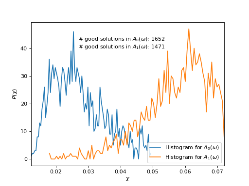
Plot \(\chi\)-histograms
from h5 import HDFArchive
from triqs.stat import Histogram
from matplotlib import pyplot as plt
from som import count_good_solutions
import numpy

# Read data from archive
ar = HDFArchive('results.h5', 'r')

hists = ar['histograms']
good_chi_abs = ar['good_chi_abs']
good_chi_rel = ar['good_chi_rel']

# Plot histograms
chi_min, chi_max = numpy.inf, 0
for n, hist in enumerate(hists):
    chi_grid = numpy.array([hist.mesh_point(n) for n in range(len(hist))])
    chi_min = min(chi_min, chi_grid[0])
    chi_max = max(chi_min, chi_grid[-1])
    plt.plot(chi_grid, hist.data, label=r"Histogram for $A_%d(\omega)$" % n)

plt.xlim((chi_min, chi_max))
plt.xlabel(r"$\chi$")
plt.ylabel(r"$P(\chi)$")
plt.legend(loc="lower right")

# Count good solutions using saved histograms
n_good_sol = [count_good_solutions(h,
                                   good_chi_abs=good_chi_abs,
                                   good_chi_rel=good_chi_rel)
              for h in hists]

plt.text(0.027, 40,
         ("# good solutions in $A_0(\\omega)$: %d\n"
          "# good solutions in $A_1(\\omega)$: %d") %
         (n_good_sol[0], n_good_sol[1]))
(Source code, png, hires.png, pdf)