Dynamical response function at zero temperature
Formally speaking, the imaginary time segment \(\tau\in[0;\beta)\) turns into an infinite interval as \(\beta\to\infty\). Similarly, spacing between Matsubara frequencies goes to 0 in that limit, and the difference between fermionic and bosonic Matsubaras disappears.
One can still define a correlation function on a finite time mesh \(\tau_i\in[0;\tau_{max}]\), and assume the function is zero for \(\tau>\tau_{max}\). In the frequency representation this corresponds to fictitious Matsubara spacing \(2\pi/\tau_{max}\).
The spectral function is defined only on the positive half-axis of energy, since \((1\pm e^{-\beta\epsilon})^{-1}\) vanishes for negative \(\epsilon\) in the zero temperature limit.
Perform analytic continuation using the ZeroTemp kernel
# Import HDFArchive and some TRIQS modules
from h5 import HDFArchive
from triqs.gf import *
import triqs.utility.mpi as mpi

# Import main SOM class and utility functions
from som import Som, fill_refreq, compute_tail, reconstruct

n_w = 1001                 # Number of energy slices for the solution
energy_window = (0, 10.0)  # Energy window to search the solution in
tail_max_order = 10        # Maximum tail expansion order to be computed

# Parameters for Som.accumulate()
acc_params = {'energy_window': energy_window}
# Verbosity level
acc_params['verbosity'] = 2
# Number of particular solutions to accumulate
acc_params['l'] = 2000
# Number of global updates
acc_params['f'] = 100
# Number of local updates per global update
acc_params['t'] = 50
# Accumulate histogram of the objective function values
acc_params['make_histograms'] = True

# Read G(\tau) from archive.
# Could be G(i\omega_n) or G_l as well.
g_tau = HDFArchive('input.h5', 'r')['g_tau']

# Set the error bars to a constant (all points of g_tau are equally important)
error_bars = g_tau.copy()
error_bars.data[:] = 0.01

# Construct a SOM object
# Norm of the spectral function is known to be 0.5.
cont = Som(g_tau, error_bars, kind="ZeroTemp", norms=[0.5])

# Accumulate particular solutions. This may take some time ...
cont.accumulate(**acc_params)

# Construct the final solution as a sum of good particular solutions with
# equal weights. Good particular solutions are those with \chi <= good_d_abs
# and \chi/\chi_{min} <= good_d_rel.
good_chi_abs = 0.002
good_chi_rel = 2.0
cont.compute_final_solution(good_chi_abs=good_chi_abs,
                            good_chi_rel=good_chi_rel,
                            verbosity=1)

# Recover G(\omega) on an energy mesh.
# NB: we can use *any* energy window at this point, not necessarily that
# from 'acc_params'.
g_w = GfReFreq(window=(0, 10.0),
               n_points=n_w,
               indices=[0])
fill_refreq(g_w, cont)

# Do the same, but this time without binning.
g_w_wo_binning = GfReFreq(window=(0, 10.0),
                          n_points=n_w,
                          indices=g_tau.indices)
fill_refreq(g_w_wo_binning, cont, with_binning=False)

# Compute tail coefficients of G(\omega)
tail = compute_tail(tail_max_order, cont)

# G(\tau) reconstructed from the solution
g_rec_tau = g_tau.copy()
reconstruct(g_rec_tau, cont)

# On master node, save parameters and results to an archive
if mpi.is_master_node():
    with HDFArchive("results.h5", 'w') as ar:
        ar['acc_params'] = acc_params
        ar['good_chi_abs'] = good_chi_abs
        ar['good_chi_rel'] = good_chi_rel
        ar['g_tau'] = g_tau
        ar['g_rec_tau'] = g_rec_tau
        ar['g_w'] = g_w
        ar['g_w_wo_binning'] = g_w_wo_binning
        ar['tail'] = tail
        ar['histograms'] = cont.histograms
Download input file input.h5.
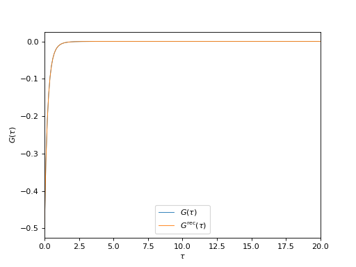
Plot input and reconstructed imaginary-time correlators
from h5 import HDFArchive
from triqs.gf import *
from matplotlib import pyplot as plt
from triqs.plot.mpl_interface import oplot

# Read data from archive
ar = HDFArchive('results.h5', 'r')

g_tau = ar['g_tau']
g_rec_tau = ar['g_rec_tau']

# Plot input and reconstructed G(\tau)
oplot(g_tau[0, 0],     mode='R', lw=0.8, label=r"$G(\tau)$")
oplot(g_rec_tau[0, 0], mode='R', lw=0.8, label=r"$G^\mathrm{rec}(\tau)$")

plt.xlim((0, g_tau.mesh.beta))
plt.ylabel(r"$G(\tau)$")
plt.legend(loc="lower center")
(Source code, png, hires.png, pdf)
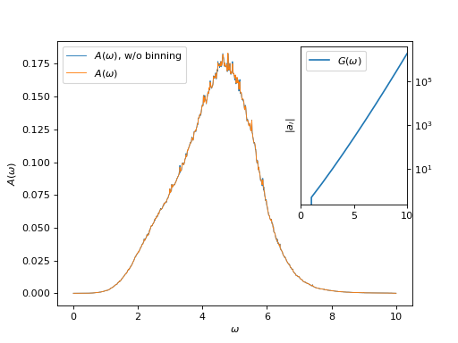
Plot spectral function and tail coefficients
from h5 import HDFArchive
from triqs.gf import *
from matplotlib import pyplot as plt
from mpl_toolkits.axes_grid1.inset_locator import inset_axes
from triqs.plot.mpl_interface import oplot
import numpy

# Read data from archive
ar = HDFArchive('results.h5', 'r')

g_w = ar['g_w']
g_w_wob = ar['g_w_wo_binning']
tail = ar['tail']

# Plot spectral functions with and without binning
oplot(g_w_wob[0, 0], mode='S', lw=0.8, label=r"$A(\omega)$, w/o binning")
oplot(g_w[0, 0], mode='S', linewidth=0.8, label=r"$A(\omega)$")

plt.ylabel(r"$A(\omega)$")
plt.legend(loc="upper left")

# Plot tail coefficients
tail_orders = numpy.array(range(tail.shape[0]))
tail_ax = inset_axes(plt.gca(), width="30%", height="60%", loc="upper right")
tail_ax.semilogy(tail_orders, numpy.abs(tail[:, 0, 0]), label=r"$G(\omega)$")
tail_ax.set_xlim((tail_orders[0], tail_orders[-1]))
tail_ax.set_ylabel("$|a_i|$")
tail_ax.yaxis.tick_right()
tail_ax.legend()
(Source code, png, hires.png, pdf)
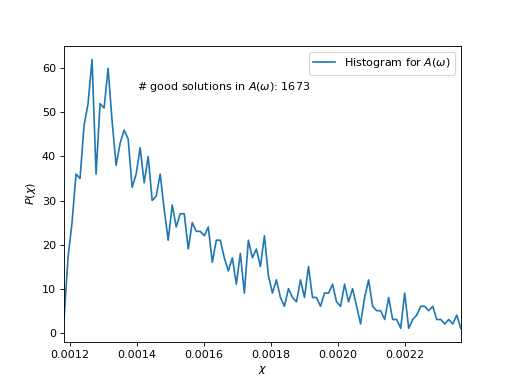
Plot \(\chi\)-histogram
from h5 import HDFArchive
from triqs.stat import Histogram
from matplotlib import pyplot as plt
from som import count_good_solutions
import numpy

# Read data from archive
ar = HDFArchive('results.h5', 'r')

hist = ar['histograms'][0]
good_chi_abs = ar['good_chi_abs']
good_chi_rel = ar['good_chi_rel']

# Plot histogram
chi_grid = numpy.array([hist.mesh_point(n) for n in range(len(hist))])
plt.plot(chi_grid, hist.data, label=r"Histogram for $A(\omega)$")

plt.xlim((chi_grid[0], chi_grid[-1]))
plt.xlabel(r"$\chi$")
plt.ylabel(r"$P(\chi)$")
plt.legend(loc="upper right")

# Count good solutions using saved histograms
n_good_sol = count_good_solutions(hist,
                                  good_chi_abs=good_chi_abs,
                                  good_chi_rel=good_chi_rel)

plt.text(0.0014, 55, "# good solutions in $A(\\omega)$: %d" % n_good_sol)
(Source code, png, hires.png, pdf)