Stochastic Optimization with Consistent Constraints
Both aspects of SOCC functionality are covered by this example: It shows how to enable the consistent-constraints updates and how to invoke the SOCC self-consistent optimization algorithm to construct the final solution.
When calculating the final solution, we use a predefined default model (“target”) and a monitor function that stores SOCC regularization parameters as they change from one iteration of the optimization process to the next.
Accumulate particular solutions and apply both SOM and SOCC procedures to construct the final solution
# Import HDFArchive, some TRIQS modules and NumPy
from h5 import HDFArchive
from triqs.gf import *
import triqs.utility.mpi as mpi
import numpy as np

# Import main SOM class and utility functions
from som import Som, fill_refreq, reconstruct

n_w = 501                    # Number of energy slices for the solution
energy_window = (-4.0, 4.0)  # Energy window to search the solution in

# Parameters for Som.accumulate()
acc_params = {'energy_window': energy_window}
# Verbosity level
acc_params['verbosity'] = 2
# Number of particular solutions to accumulate
acc_params['l'] = 200
# Number of global updates
acc_params['f'] = 100
# Number of local updates per global update
acc_params['t'] = 200
# Enable CC updates
acc_params['cc_update'] = True
# Two consecutive CC updates are separated by this number of elementary updates
acc_params['cc_update_cycle_length'] = 20

# Read g(\tau) from an archive.
with HDFArchive('input.h5', 'r') as ar:
    g_tau = ar['g_tau']

# Set the error bars to a constant
error_bars = g_tau.copy()
error_bars.data[:] = 0.001

# Construct a SOM object
cont = Som(g_tau, error_bars, kind="FermionGfSymm")

# Accumulate particular solutions
cont.accumulate(**acc_params)

#
# Use the standard SOM procedure to construct the final solution and to compute
# the value it delivers to the \chi^2 functional.
#

chi2 = cont.compute_final_solution(good_chi_rel=4.0, verbosity=1)

# Recover g(\omega) on an energy mesh
g_w = GfReFreq(window=energy_window, n_points=n_w, indices=[0])
fill_refreq(g_w, cont)

# g(\tau) reconstructed from the solution
g_rec_tau = g_tau.copy()
reconstruct(g_rec_tau, cont)

# On master node, save results to an archive
if mpi.is_master_node():
    with HDFArchive("results.h5", 'a') as ar:
        ar.create_group("som")
        gr = ar["som"]
        gr['g_tau'] = g_tau
        gr['chi2'] = chi2
        gr['g_w'] = g_w
        gr['g_rec_tau'] = g_rec_tau

#
# Use the SOCC protocol to construct the final solution and to compute
# the value it delivers to the \chi^2 functional.
#

# Real frequency mesh to be used in the SOCC optimization protocol
refreq_mesh = MeshReFreq(*energy_window, n_w)

# Parameters of compute_final_solution_cc()
params = {'refreq_mesh': refreq_mesh}
params['good_chi_rel'] = 4.0
params['verbosity'] = 1

# One can optionally provide a target (default) model so that the final solution
# is 'pulled' towards it. Here, we use a Gaussian spectral function.
default_model = np.array([np.exp(-(float(e) ** 2) / 2) / np.sqrt(2*np.pi)
                          for e in refreq_mesh])
params['default_model'] = default_model
# Set importance of the default model equal for all real energy points.
params['default_model_weights'] = 1e-2 * np.ones(n_w)

# Monitor function for compute_final_solution_cc().
#
# It saves expansion coefficients of the final solution, magnitudes and
# derivatives of the solution, and values of the regularization parameters at
# each CC iteration.
cc_iterations = []


def monitor_f(c, AQ, ApD, AppB):
    if mpi.rank == 0:
        A_k, Q_k = AQ
        Ap_k, D_k = ApD
        App_k, B_k = AppB
        cc_iterations.append({'c': c,
                              'A_k': A_k, 'Q_k': Q_k,
                              'Ap_k': Ap_k, 'D_k': D_k,
                              'App_k': App_k, 'B_k': B_k})
    # Returning 'True' would instruct compute_final_solution_cc() to
    # terminate iterations.
    return False


params['monitor'] = monitor_f

# Various fine-tuning options
params['max_iter'] = 20
params['ew_penalty_coeff'] = 1.0
params['amp_penalty_max'] = 1e3
params['amp_penalty_divisor'] = 10.0
params['der_penalty_init'] = 0.1
params['der_penalty_coeff'] = 2.0

chi2 = cont.compute_final_solution_cc(**params)

# Recover g(\omega) on an energy mesh
g_w = GfReFreq(window=energy_window, n_points=n_w, indices=[0])
fill_refreq(g_w, cont)

# g(\tau) reconstructed from the solution
g_rec_tau = g_tau.copy()
reconstruct(g_rec_tau, cont)

# On master node, save results to an archive
if mpi.is_master_node():
    with HDFArchive("results.h5", 'a') as ar:
        ar.create_group("socc")
        gr = ar["socc"]
        gr['g_tau'] = g_tau
        gr['default_model'] = default_model
        gr['chi2'] = chi2
        gr['g_w'] = g_w
        gr['g_rec_tau'] = g_rec_tau
        gr['iterations'] = cc_iterations
Plot spectral functions, reconstructed Green’s functions and evolution of SOCC regularization parameters
from h5 import HDFArchive
from triqs.gf import Gf # noqa: F401
from matplotlib import pyplot as plt
from matplotlib.colors import LogNorm
from triqs.plot.mpl_interface import oplot
import numpy as np
# Read data from archive
ar = HDFArchive("results.h5", 'r')
# Energy mesh
energy_mesh = ar["som"]["g_w"].mesh
w_points = np.array([float(w) for w in energy_mesh])
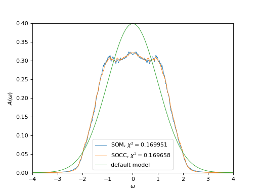
# Plot spectral functions obtained using SOM and SOCC procedures
oplot(ar["som"]["g_w"], mode='S', lw=0.8,
label=r'SOM, $\chi^2=%f$' % ar["som"]["chi2"][0])
oplot(ar["socc"]["g_w"], mode='S', lw=0.8,
label=r'SOCC, $\chi^2=%f$' % ar["socc"]["chi2"][0])
# Plot the default model
plt.plot(w_points, ar["socc"]["default_model"], lw=0.8,
label="default model")
plt.xlim((energy_mesh.w_min, energy_mesh.w_max))
plt.ylim((0, 0.4))
plt.ylabel(r"$A(\omega)$")
plt.legend()
plt.show()
(Source code, png, hires.png, pdf)
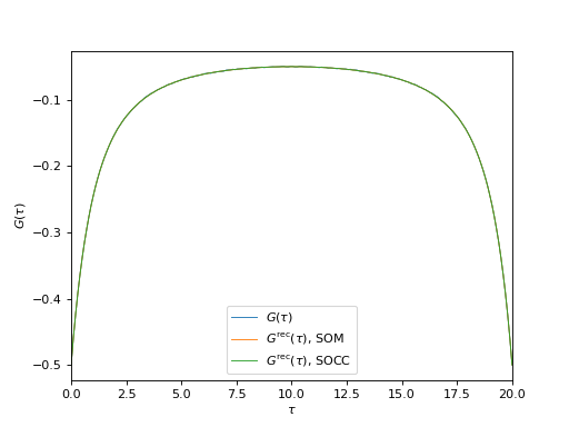
# Plot input and reconstructed G(\tau)
oplot(ar["som"]["g_tau"][0, 0], mode='R', lw=0.8, label=r"$G(\tau)$")
oplot(ar["som"]["g_rec_tau"][0, 0], mode='R', lw=0.8,
      label=r"$G^\mathrm{rec}(\tau)$, SOM")
oplot(ar["socc"]["g_rec_tau"][0, 0], mode='R', lw=0.8,
      label=r"$G^\mathrm{rec}(\tau)$, SOCC")

plt.xlim((0, ar["som"]["g_tau"].mesh.beta))
plt.ylabel(r"$G(\tau)$")
plt.legend(loc="lower center")
plt.show()
#
# Plot evolution of SOCC regularization parameters with iterations
#
socc_iterations = ar['socc']['iterations']
N_iter = len(socc_iterations)
N_k = len(socc_iterations[0]['Q_k'])
A_k, Q_k = np.zeros((N_k, N_iter)), np.zeros((N_k, N_iter))
Ap_k, D_k = np.zeros((N_k - 1, N_iter)), np.zeros((N_k - 1, N_iter))
App_k, B_k = np.zeros((N_k - 2, N_iter)), np.zeros((N_k - 2, N_iter))
for i, it in enumerate(socc_iterations):
A_k[:, i] = it['A_k']
Q_k[:, i] = it['Q_k']
Ap_k[:, i] = it['Ap_k']
D_k[:, i] = it['D_k']
App_k[:, i] = it['App_k']
B_k[:, i] = it['B_k']
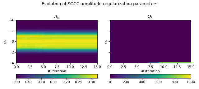
# Amplitude regularization parameters
fig, axes = plt.subplots(1, 2, sharey='row', figsize=(8, 3.6))
fig.suptitle("Evolution of SOCC amplitude regularization parameters")
A_k_image = axes[0].imshow(A_k, extent=(0, N_iter, w_points[-1], w_points[0]))
axes[0].set_title(r"$A_k$")
axes[0].set_xlabel(r"# iteration")
axes[0].set_ylabel(r"$\omega_k$")
plt.colorbar(A_k_image, ax=axes[0], orientation='horizontal')
Q_k_image = axes[1].imshow(Q_k, extent=(0, N_iter, w_points[-1], w_points[0]))
axes[1].set_title(r"$Q_k$")
axes[1].set_xlabel(r"# iteration")
axes[1].set_ylabel(r"$\omega_k$")
plt.colorbar(Q_k_image,
ax=axes[1],
orientation='horizontal',
norm=LogNorm(vmin=Q_k.min(), vmax=Q_k.max()))
plt.tight_layout()
plt.show()
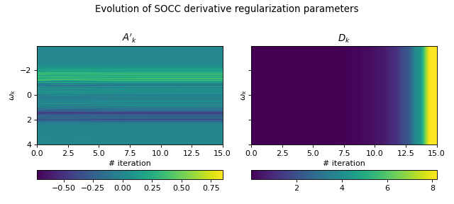
# Derivative regularization parameters
fig, axes = plt.subplots(1, 2, sharey='row', figsize=(8, 3.6))
fig.suptitle("Evolution of SOCC derivative regularization parameters")

Ap_k_image = axes[0].imshow(Ap_k, extent=(0, N_iter, w_points[-1], w_points[1]))
axes[0].set_title(r"$A'_k$")
axes[0].set_xlabel(r"# iteration")
axes[0].set_ylabel(r"$\omega_k$")
plt.colorbar(Ap_k_image, ax=axes[0], orientation='horizontal')

D_k_image = axes[1].imshow(D_k, extent=(0, N_iter, w_points[-1], w_points[1]))
axes[1].set_title(r"$D_k$")
axes[1].set_xlabel(r"# iteration")
axes[1].set_ylabel(r"$\omega_k$")
plt.colorbar(D_k_image,
             ax=axes[1],
             orientation='horizontal',
             norm=LogNorm(vmin=D_k.min(), vmax=D_k.max()))

plt.tight_layout()
plt.show()
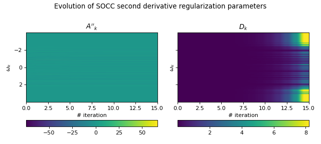
# Second derivative regularization parameters
fig, axes = plt.subplots(1, 2, sharey='row', figsize=(8, 3.6))
fig.suptitle("Evolution of SOCC second derivative regularization parameters")

App_k_image = axes[0].imshow(App_k,
                             extent=(0, N_iter, w_points[-2], w_points[1]))
axes[0].set_title(r"$A''_k$")
axes[0].set_xlabel(r"# iteration")
axes[0].set_ylabel(r"$\omega_k$")
plt.colorbar(App_k_image, ax=axes[0], orientation='horizontal')

B_k_image = axes[1].imshow(B_k, extent=(0, N_iter, w_points[-2], w_points[1]))
axes[1].set_title(r"$D_k$")
axes[1].set_xlabel(r"# iteration")
axes[1].set_ylabel(r"$\omega_k$")
plt.colorbar(B_k_image,
             ax=axes[1],
             orientation='horizontal',
             norm=LogNorm(vmin=B_k.min(), vmax=B_k.max()))

plt.tight_layout()
plt.show()