Full covariance matrix of input data

This example demonstrates three ways to provide information about uncertainty of input data (here, of an imaginary time fermionic Green’s function \(G(\tau)\)),

As estimated error bars \(\sigma(\tau)\);
As a full covariance matrix \(\hat\Sigma_{\tau\tau'}\) ;
As a full covariance matrix \(\hat\Sigma_{\tau\tau'}\) with all eigenvalues shifted up by a constant \(l^2\), where \(l\) is so called filtering level.

Perform analytic continuation

# Import HDFArchive, some TRIQS modules and NumPy
from h5 import HDFArchive
from triqs.gf import *
import triqs.utility.mpi as mpi
import numpy as np

# Import main SOM class and utility functions
from som import Som, fill_refreq, reconstruct

n_w = 801                    # Number of energy slices for G(\omega)
energy_window = (-4.0, 4.0)  # Energy window to search solutions in

# Parameters for Som.accumulate()
acc_params = {'energy_window': energy_window}
acc_params['verbosity'] = 2  # Verbosity level
acc_params['l'] = 1000       # Number of particular solutions to accumulate
acc_params['f'] = 100        # Number of global updates
acc_params['t'] = 50         # Number of local updates per global update

# Read G(\tau) from an archive.
g_tau = HDFArchive('input.h5', 'r')['g_tau']
n_tau = len(g_tau.mesh)

# Estimated error bars on all slices of 'g_tau'
sigma = 0.01

#
# Construct a Som object using the estimated error bars.
#

error_bars = g_tau.copy()
error_bars.data[:] = sigma

cont_eb = Som(g_tau, error_bars, kind="FermionGf")

#
# Construct a Som object using a full covariance matrix.
#

# Create a GF container for the covariance matrix.
# It is defined on an 'n_tau x n_tau' mesh and has a 1D target shape
# with each target element corresponding to one diagonal element of 'g_tau'.
cov_matrix = Gf(mesh=MeshProduct(g_tau.mesh, g_tau.mesh),
                target_shape=(g_tau.target_shape[0],))

# Diagonal covariance matrix equivalent to using 'error_bars'
cov_matrix.data[:, :, 0] = (sigma ** 2) * np.eye(n_tau)
# Add slight correlations between adjacent \tau-slices
cov_matrix.data[:, :, 0] += np.diag(0.00005 * np.ones(n_tau-1), k=1)
cov_matrix.data[:, :, 0] += np.diag(0.00005 * np.ones(n_tau-1), k=-1)

cont_cm = Som(g_tau, cov_matrix, kind="FermionGf")

#
# Construct a Som object using the same covariance matrix and a finite filtering
# level.
#

# Before using the covariance matrix, SOM will shift its eigenvalues up by fl^2.
fl = 0.01
cont_cmfl = Som(g_tau, cov_matrix, kind="FermionGf", filtering_levels=[fl])

#
# Perform analytic continuation
#

for name, cont in (("error_bars", cont_eb),
                   ("cov_matrix", cont_cm),
                   ("cov_matrix_fl", cont_cmfl)):
    cont.accumulate(**acc_params)
    cont.compute_final_solution(verbosity=1)

    # Recover G(\omega) on an energy mesh
    g_w = GfReFreq(window=energy_window, n_points=n_w, indices=g_tau.indices)
    fill_refreq(g_w, cont)

    # G(\tau) reconstructed from the solution
    g_rec_tau = g_tau.copy()
    reconstruct(g_rec_tau, cont)

    # On master node, save results to an archive
    if mpi.is_master_node():
        with HDFArchive("results.h5", 'a') as ar:
            ar.create_group(name)
            gr = ar[name]
            gr['g_tau'] = g_tau
            gr['g_w'] = g_w
            gr['g_rec_tau'] = g_rec_tau

Download input file input.h5.

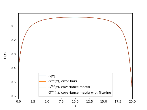
Plot input and reconstructed imaginary-time GF’s

from h5 import HDFArchive
from triqs.gf import *
from matplotlib import pyplot as plt
from triqs.plot.mpl_interface import oplot

# Read data from archive
ar = HDFArchive('results.h5', 'r')

g_tau = ar['error_bars']['g_tau']

# Plot input and reconstructed G(\tau)
oplot(g_tau, mode='R', lw=0.8, label=r"$G(\tau)$")
oplot(ar['error_bars']['g_rec_tau'][0, 0], mode='R', lw=0.8,
      label=r"$G^{rec}(\tau)$, error bars")
oplot(ar['cov_matrix']['g_rec_tau'][0, 0], mode='R', lw=0.8,
      label=r"$G^{rec}(\tau)$, covariance matrix")
oplot(ar['cov_matrix_fl']['g_rec_tau'][0, 0], mode='R', lw=0.8,
      label=r"$G^{rec}(\tau)$, covariance matrix with filtering")

plt.xlim((0, g_tau.mesh.beta))
plt.ylabel(r"$G(\tau)$")
plt.legend(loc="lower center")

(Source code, png, hires.png, pdf)

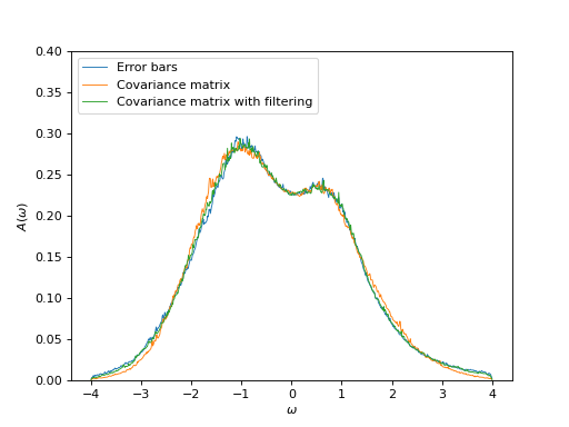
Plot spectral functions

from h5 import HDFArchive
from triqs.gf import *
from matplotlib import pyplot as plt
from triqs.plot.mpl_interface import oplot

# Read data from archive
ar = HDFArchive('results.h5', 'r')

# Plot spectral functions
oplot(ar['error_bars']['g_w'][0, 0],
      mode='S', lw=0.8, label=r"Error bars")
oplot(ar['cov_matrix']['g_w'][0, 0],
      mode='S', lw=0.8, label=r"Covariance matrix")
oplot(ar['cov_matrix_fl']['g_w'][0, 0],
      mode='S', lw=0.8, label=r"Covariance matrix with filtering")

plt.ylim((0, 0.4))
plt.ylabel(r"$A(\omega)$")
plt.legend(loc="upper left")

(Source code, png, hires.png, pdf)