Input data defined on various meshes
In this example we analytically continue the same dynamical susceptibility \(\chi\), whose values are given on three different meshes:
Bosonic
Matsubara frequencies;Points of an
imaginary time grid;Indices of
Legendre orthogonal polynomials.
# Import HDFArchive and some TRIQS modules
from h5 import HDFArchive
from triqs.gf import *
import triqs.utility.mpi as mpi

# Import main SOM class and utility functions
from som import (Som,
                 fill_refreq,
                 compute_tail,
                 reconstruct,
                 estimate_boson_corr_spectrum_norms)

n_w = 501                    # Number of energy slices for the solution
energy_window = (-4.0, 4.0)  # Energy window to search the solution in
tail_max_order = 10          # Maximum tail expansion order to be computed

# Parameters for Som.accumulate()
acc_params = {'energy_window': energy_window}
acc_params['verbosity'] = 2  # Verbosity level
acc_params['l'] = 2000       # Number of particular solutions to accumulate
acc_params['f'] = 100        # Number of global updates
acc_params['t'] = 50         # Number of local updates per global update

# Read \chi(i\Omega_n), \chi(\tau) and \chi_l from an archive.
with HDFArchive('input.h5', 'r') as ar:
    chi_iw = ar['chi_iw']
    chi_tau = ar['chi_tau']
    chi_l = ar['chi_l']

#
# Analytically continue \chi(i\Omega_n), \chi(\tau) and \chi_l
#

for mesh_name, chi in (("ImFreq", chi_iw),
                       ("ImTime", chi_tau),
                       ("Legendre", chi_l)):

    # Estimate norms of spectral functions from input data
    norms = estimate_boson_corr_spectrum_norms(chi)

    # Set the error bars to a constant
    error_bars = chi.copy()
    error_bars.data[:] = 0.001

    # Construct a SOM object
    cont = Som(chi, error_bars, kind="BosonAutoCorr", norms=norms)

    # Accumulate particular solutions
    cont.accumulate(**acc_params)

    # Construct the final solution
    cont.compute_final_solution(good_chi_rel=4.0, verbosity=1)

    # Recover \chi(\omega) on an energy mesh.
    chi_w = GfReFreq(window=energy_window, n_points=n_w, indices=chi.indices)
    fill_refreq(chi_w, cont)

    # \chi reconstructed from the solution
    chi_rec = chi.copy()
    reconstruct(chi_rec, cont)

    # On master node, save results to an archive
    if mpi.is_master_node():
        with HDFArchive("results.h5", 'a') as ar:
            ar.create_group(mesh_name)
            gr = ar[mesh_name]
            gr['norms'] = norms
            gr['chi'] = chi
            gr['chi_w'] = chi_w
            gr['chi_rec'] = chi_rec
Download input file input.h5.
Plot input and reconstructed susceptibility
from h5 import HDFArchive
from triqs.gf import *
from matplotlib import pyplot as plt
from triqs.plot.mpl_interface import oplot
# Read data from archive
ar = HDFArchive('results.h5', 'r')
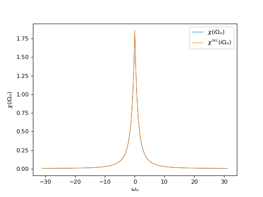
# Plot input and reconstructed \chi(i\Omega_n)
oplot(ar['ImFreq']['chi'][0, 0], mode='R', lw=0.8, label=r"$\chi(i\Omega_n)$")
oplot(ar['ImFreq']['chi_rec'][0, 0], mode='R', lw=0.8,
label=r"$\chi^{rec}(i\Omega_n)$")
plt.ylabel(r"$\chi(i\Omega_n)$")
plt.legend(loc="upper right")
plt.show()
(Source code, png, hires.png, pdf)
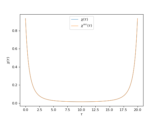
# Plot input and reconstructed \chi(\tau)
oplot(ar['ImTime']['chi'][0, 0], mode='R', lw=0.8, label=r"$\chi(\tau)$")
oplot(ar['ImTime']['chi_rec'][0, 0], mode='R', lw=0.8,
      label=r"$\chi^{rec}(\tau)$")

plt.ylabel(r"$\chi(\tau)$")
plt.legend(loc="upper center")
plt.show()
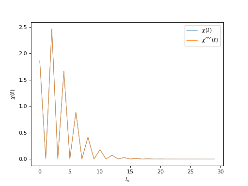
# Plot input and reconstructed \chi(\ell)
oplot(ar['Legendre']['chi'][0, 0], mode='R', lw=0.8, label=r"$\chi(\ell)$")
oplot(ar['Legendre']['chi_rec'][0, 0], mode='R', lw=0.8,
      label=r"$\chi^{rec}(\ell)$")

plt.ylabel(r"$\chi(\ell)$")
plt.legend(loc="upper right")
plt.show()
Plot spectral functions
from h5 import HDFArchive
from triqs.gf import *
from matplotlib import pyplot as plt
from triqs.plot.mpl_interface import oplot
# Read data from archive
ar = HDFArchive('results.h5', 'r')
#
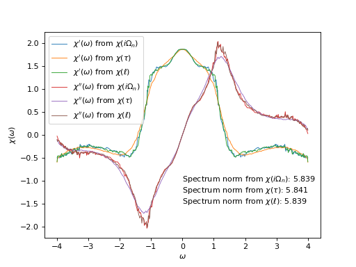
# Plot susceptibility as a function of real frequencies
#
# Real parts
oplot(ar['ImFreq']['chi_w'][0, 0],
mode='R', lw=0.8, label=r"$\chi'(\omega)$ from $\chi(i\Omega_n)$")
oplot(ar['ImTime']['chi_w'][0, 0],
mode='R', lw=0.8, label=r"$\chi'(\omega)$ from $\chi(\tau)$")
oplot(ar['Legendre']['chi_w'][0, 0],
mode='R', lw=0.8, label=r"$\chi'(\omega)$ from $\chi(\ell)$")
# Imaginary parts
oplot(ar['ImFreq']['chi_w'][0, 0],
mode='I', lw=0.8, label=r"$\chi''(\omega)$ from $\chi(i\Omega_n)$")
oplot(ar['ImTime']['chi_w'][0, 0],
mode='I', lw=0.8, label=r"$\chi''(\omega)$ from $\chi(\tau)$")
oplot(ar['Legendre']['chi_w'][0, 0],
mode='I', lw=0.8, label=r"$\chi''(\omega)$ from $\chi(\ell)$")
# Spectrum normalization constants extracted from input data
norms_text = [
r"Spectrum norm from $\chi(i\Omega_n)$: %.3f" % ar['ImFreq']['norms'][0],
r"Spectrum norm from $\chi(\tau)$: %.3f" % ar['ImTime']['norms'][0],
r"Spectrum norm from $\chi(\ell)$: %.3f" % ar['Legendre']['norms'][0]
]
norms_text = "\n".join(norms_text)
plt.text(0, -1.5, norms_text)
plt.ylabel(r"$\chi(\omega)$")
plt.legend(loc="upper left")
(Source code, png, hires.png, pdf)