Green’s function of bosons and transverse magnetic susceptibility
A general correlation function of boson-like operators \(\hat O\) and \(\hat O^\dagger\) is defined as
\[\chi(\tau) = \langle\mathbb{T}_\tau \hat O(\tau) \hat O^\dagger(0)\rangle.\]
\(\chi(\tau)\) is subject to the periodicity condition
\[\chi(\tau+\beta) = \chi(\tau).\]
Examples of such correlators are the transverse magnetic susceptibility \(\langle\mathbb{T}_\tau \hat S_+(\tau) \hat S_-(0)\rangle\) and the Green’s function of bosons \(\langle\mathbb{T}_\tau \hat b(\tau) \hat b^\dagger(0)\rangle\).
The auxiliary spectral function \(A(\epsilon) = \Im\chi(\epsilon)/\epsilon\) is non-negative but not necessarily symmetric.
Warning
When \(\hat O = \hat O^\dagger\) (for instance, in the case of charge or longitudinal magnetic susceptibility), it is strongly recommended to use the BosonAutoCorr observable kind instead of BosonCorr shown here.
Perform analytic continuation using the BosonCorr kernel
# Import HDFArchive and some TRIQS modules
from h5 import HDFArchive
from triqs.gf import *
import triqs.utility.mpi as mpi

# Import main SOM class and utility functions
from som import Som, fill_refreq, compute_tail, reconstruct

n_w = 1001                   # Number of energy slices for the solution
energy_window = (-5.0, 5.0)  # Energy window to search the solution in
tail_max_order = 10          # Maximum tail expansion order to be computed

# Parameters for Som.accumulate()
acc_params = {'energy_window': energy_window}
# Verbosity level
acc_params['verbosity'] = 2
# Number of particular solutions to accumulate
acc_params['l'] = 2000
# Number of global updates
acc_params['f'] = 100
# Number of local updates per global update
acc_params['t'] = 50
# Accumulate histogram of the objective function values
acc_params['make_histograms'] = True
# Right boundary of the histogram, in units of \chi_{min}
acc_params['hist_max'] = 4.0

# Read \chi(i\omega_n) from archive.
# Could be \chi(\tau) or \chi_l as well.
chi_iw = HDFArchive('input.h5', 'r')['chi_iw']

# Set the error bars to a constant (all points of chi_iw are equally important)
error_bars = chi_iw.copy()
error_bars.data[:] = 0.001

# Construct a SOM object
# Norms of spectral functions are known to be 3.0 for both diagonal components
# of chi_iw. It would also be possible to estimate the norms by calling
# som.estimate_boson_corr_spectrum_norms(chi_iw).
cont = Som(chi_iw, error_bars, kind="BosonCorr", norms=[3.0, 3.0])

# Accumulate particular solutions. This may take some time ...
cont.accumulate(**acc_params)

# Construct the final solution as a sum of good particular solutions with
# equal weights. Good particular solutions are those with \chi <= good_d_abs
# and \chi/\chi_{min} <= good_d_rel.
good_chi_abs = 1.0
good_chi_rel = 4.0
cont.compute_final_solution(good_chi_abs=good_chi_abs,
                            good_chi_rel=good_chi_rel,
                            verbosity=1)

# Recover \chi(\omega) on an energy mesh.
# NB: we can use *any* energy window at this point, not necessarily that
# from 'acc_params'.
chi_w = GfReFreq(window=(-5.0, 5.0),
                 n_points=n_w,
                 indices=chi_iw.indices)
fill_refreq(chi_w, cont)

# Do the same, but this time without binning.
chi_w_wo_binning = GfReFreq(window=(-5.0, 5.0),
                            n_points=n_w,
                            indices=chi_iw.indices)
fill_refreq(chi_w_wo_binning, cont, with_binning=False)

# Compute tail coefficients of \chi(\omega)
tail = compute_tail(tail_max_order, cont)

# \chi(i\omega) reconstructed from the solution
chi_rec_iw = chi_iw.copy()
reconstruct(chi_rec_iw, cont)

# On master node, save parameters and results to an archive
if mpi.is_master_node():
    with HDFArchive("results.h5", 'w') as ar:
        ar['acc_params'] = acc_params
        ar['good_chi_abs'] = good_chi_abs
        ar['good_chi_rel'] = good_chi_rel
        ar['chi_iw'] = chi_iw
        ar['chi_rec_iw'] = chi_rec_iw
        ar['chi_w'] = chi_w
        ar['chi_w_wo_binning'] = chi_w_wo_binning
        ar['tail'] = tail
        ar['histograms'] = cont.histograms
Download input file input.h5.
Plot input and reconstructed correlators at Matsubara frequencies
from h5 import HDFArchive
from triqs.gf import *
from matplotlib import pyplot as plt
from triqs.plot.mpl_interface import oplot
# Read data from archive
ar = HDFArchive('results.h5', 'r')
chi_iw = ar['chi_iw']
chi_rec_iw = ar['chi_rec_iw']
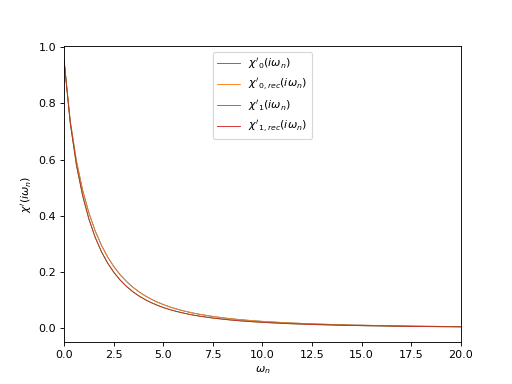
# Plot real part of input and reconstructed \chi(i\omega_n)
oplot(chi_iw[0, 0], mode='R', lw=0.8, label=r"$\chi'_0(i\omega_n)$")
oplot(chi_rec_iw[0, 0], mode='R', lw=0.8, label=r"$\chi'_{0,rec}(i\omega_n)$")
oplot(chi_iw[1, 1], mode='R', lw=0.8, label=r"$\chi'_1(i\omega_n)$")
oplot(chi_rec_iw[1, 1], mode='R', lw=0.8, label=r"$\chi'_{1,rec}(i\omega_n)$")
plt.xlim((0, 20.0))
plt.ylabel(r"$\chi'(i\omega_n)$")
plt.legend(loc="upper center")
plt.show()
(Source code, png, hires.png, pdf)
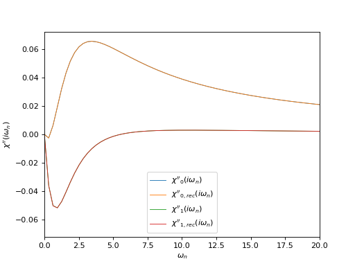
# Plot imaginary part of input and reconstructed \chi(i\omega_n)
oplot(chi_iw[0, 0],     mode='I', lw=0.8, label=r"$\chi''_0(i\omega_n)$")
oplot(chi_rec_iw[0, 0], mode='I', lw=0.8, label=r"$\chi''_{0,rec}(i\omega_n)$")
oplot(chi_iw[1, 1],     mode='I', lw=0.8, label=r"$\chi''_1(i\omega_n)$")
oplot(chi_rec_iw[1, 1], mode='I', lw=0.8, label=r"$\chi''_{1,rec}(i\omega_n)$")

plt.xlim((0, 20.0))
plt.ylabel(r"$\chi''(i\omega_n)$")
plt.legend(loc="lower center")
Plot the correlator on the real frequency axis and its tail coefficients
from h5 import HDFArchive
from triqs.gf import *
from matplotlib import pyplot as plt
from triqs.plot.mpl_interface import oplot
# Read data from archive
ar = HDFArchive('results.h5', 'r')
chi_w = ar['chi_w']
chi_w_wob = ar['chi_w_wo_binning']
tail = ar['tail']
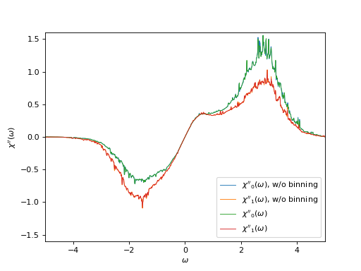
# Plot imaginary part of the correlator on the real axis
# with and without binning
oplot(chi_w_wob[0, 0],
mode='I', lw=0.8, label=r"$\chi''_0(\omega)$, w/o binning")
oplot(chi_w_wob[1, 1],
mode='I', lw=0.8, label=r"$\chi''_1(\omega)$, w/o binning")
oplot(chi_w[0, 0], mode='I', lw=0.8, label=r"$\chi''_0(\omega)$")
oplot(chi_w[1, 1], mode='I', lw=0.8, label=r"$\chi''_1(\omega)$")
plt.xlim((-5.0, 5.0))
plt.ylim((-1.6, 1.6))
plt.ylabel(r"$\chi''(\omega)$")
plt.legend(loc="lower right")
(Source code, png, hires.png, pdf)
Plot \(\chi\)-histograms
from h5 import HDFArchive
from triqs.stat import Histogram
from matplotlib import pyplot as plt
from som import count_good_solutions
import numpy
# Read data from archive
ar = HDFArchive('results.h5', 'r')
hists = ar['histograms']
good_chi_abs = ar['good_chi_abs']
good_chi_rel = ar['good_chi_rel']
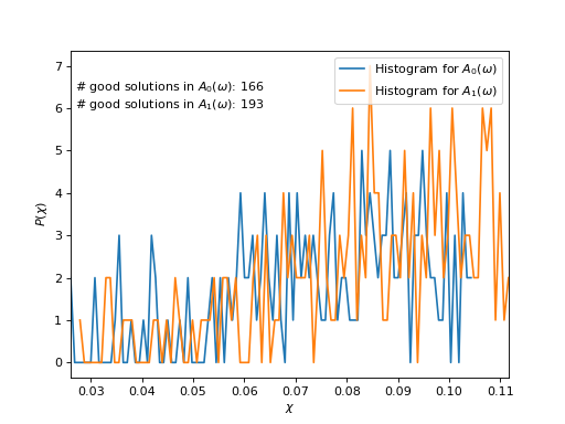
# Plot histograms
chi_min, chi_max = numpy.inf, 0
for n, hist in enumerate(hists):
chi_grid = numpy.array([hist.mesh_point(n) for n in range(len(hist))])
chi_min = min(chi_min, chi_grid[0])
chi_max = max(chi_min, chi_grid[-1])
plt.plot(chi_grid, hist.data, label=r"Histogram for $A_%d(\omega)$" % n)
plt.xlim((chi_min, chi_max))
plt.xlabel(r"$\chi$")
plt.ylabel(r"$P(\chi)$")
plt.legend(loc="upper right")
# Count good solutions using saved histograms
n_good_sol = [count_good_solutions(h,
good_chi_abs=good_chi_abs,
good_chi_rel=good_chi_rel)
for h in hists]
print(hists[0])
plt.text(0.027, 6,
("# good solutions in $A_0(\\omega)$: %d\n"
"# good solutions in $A_1(\\omega)$: %d") %
(n_good_sol[0], n_good_sol[1]))
(Source code, png, hires.png, pdf)