Statistical analysis of ensembles of spectral functions
This example is an illustration of the spectral statistical analysis API. In the script below, we use the same input data for a two-component fermionic Green’s function as in another example, but never construct a final solution out of accumulated particular solutions. Instead, we estimate it by computing spectral averages over the ensemble of the particular solutions, along with error bars (dispersions) and two-point correlations. Use of all three resolution functions is shown.
Accumulate particular solutions and compute statistical characteristics
# Import HDFArchive and some TRIQS modules
from h5 import HDFArchive
from triqs.gf import *
import triqs.utility.mpi as mpi

# Import main SOM class
from som import Som
# Import statistical analysis functions
from som.spectral_stats import spectral_avg, spectral_disp, spectral_corr

energy_window = (-4.0, 4.0)  # Energy window to search the solution in

# Parameters for Som.accumulate()
acc_params = {'energy_window': energy_window}
acc_params['verbosity'] = 2  # Verbosity level
acc_params['l'] = 1000       # Number of particular solutions to accumulate
acc_params['f'] = 100        # Number of global updates
acc_params['t'] = 50         # Number of local updates per global update

# Read G(\tau) from an archive.
g_tau = HDFArchive('input.h5', 'r')['g_tau']

# Set the error bars to a constant (all points of g_tau are equally important)
error_bars = g_tau.copy()
error_bars.data[:] = 0.01

# Construct a SOM object
cont = Som(g_tau, error_bars, kind="FermionGf")

# Accumulate particular solutions. This may take some time ...
cont.accumulate(**acc_params)

#
# Compute statistical characteristics of the ensemble of the accumulated
# particular solutions.
#

# We use a set of energy intervals centered around points of this mesh
w_mesh = MeshReFreq(*energy_window, 401)

for i in (0, 1):
    # Compute spectral averages using different resolution functions.
    avg_rect = spectral_avg(cont, i, w_mesh, "rectangle")
    avg_lorentz = spectral_avg(cont, i, w_mesh, "lorentzian")
    avg_gauss = spectral_avg(cont, i, w_mesh, "gaussian")

    # Compute spectral dispersions using different resolution functions.
    disp_rect = spectral_disp(cont, i, w_mesh, avg_rect, "rectangle")
    disp_lorentz = spectral_disp(cont, i, w_mesh, avg_lorentz, "lorentzian")
    disp_gauss = spectral_disp(cont, i, w_mesh, avg_gauss, "gaussian")

    # Compute two-point correlators using different resolution functions.
    corr_rect = spectral_corr(cont, i, w_mesh, avg_rect, "rectangle")
    corr_lorentz = spectral_corr(cont, i, w_mesh, avg_lorentz, "lorentzian")
    corr_gauss = spectral_corr(cont, i, w_mesh, avg_gauss, "gaussian")

    # On master node, save results to an archive
    if mpi.is_master_node():
        with HDFArchive("results.h5", 'a') as ar:
            ar.create_group(str(i))
            gr = ar[str(i)]
            gr['w_mesh'] = w_mesh
            gr['avg_rect'] = avg_rect
            gr['avg_lorentz'] = avg_lorentz
            gr['avg_gauss'] = avg_gauss
            gr['disp_rect'] = disp_rect
            gr['disp_lorentz'] = disp_lorentz
            gr['disp_gauss'] = disp_gauss
            gr['corr_rect'] = corr_rect
            gr['corr_lorentz'] = corr_lorentz
            gr['corr_gauss'] = corr_gauss
Download input file input.h5.
Plot statistical characteristics
from h5 import HDFArchive
from triqs.gf import *
from matplotlib import pyplot as plt
import numpy as np
# Read data from archive
ar = HDFArchive('results.h5', 'r')
w_mesh = ar["0"]["w_mesh"]
w_points = np.array([float(w) for w in w_mesh])
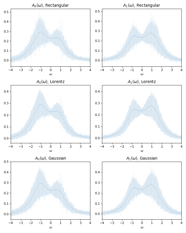
#
# Plot averaged spectra with error bars derived from estimated dispersions
#
fig, axes = plt.subplots(3, 2, figsize=(8, 10))
for i in (0, 1):
gr = ar[str(i)]
# Rectangular resolution function
axes[0, i].errorbar(w_points,
gr["avg_rect"],
xerr=w_mesh.delta,
yerr=np.sqrt(gr["disp_rect"]),
lw=0.1)
axes[0, i].set_title(r"$A_%d(\omega)$, Rectangular" % i)
# Lorentzian resolution function
axes[1, i].errorbar(w_points,
gr["avg_lorentz"],
xerr=w_mesh.delta,
yerr=np.sqrt(gr["disp_lorentz"]),
lw=0.1)
axes[1, i].set_title(r"$A_%d(\omega)$, Lorentz" % i)
# Gaussian resolution function
axes[2, i].errorbar(w_points,
gr["avg_gauss"],
xerr=w_mesh.delta,
yerr=np.sqrt(gr["disp_gauss"]),
lw=0.1)
axes[2, i].set_title(r"$A_%d(\omega)$, Gaussian" % i)
plt.setp(axes, xlim=(w_points[0], w_points[-1]), xlabel=r"$\omega$")
plt.tight_layout()
plt.show()
(Source code, png, hires.png, pdf)
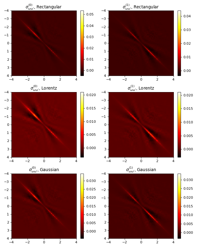
#
# Plot two-point correlators
#

fig, axes = plt.subplots(3, 2, figsize=(8, 10))
for i in (0, 1):
    gr = ar[str(i)]

    extent = [w_points[0], w_points[-1], w_points[-1], w_points[0]]

    # Rectangular resolution function
    corr = axes[0, i].imshow(gr["corr_rect"], extent=extent, cmap="hot")
    fig.colorbar(corr, ax=axes[0, i])
    axes[0, i].set_title(r"$\sigma_{\omega\omega'}^{(%d)}$, Rectangular" % i)

    # Lorentzian resolution function
    corr = axes[1, i].imshow(gr["corr_lorentz"], extent=extent, cmap="hot")
    fig.colorbar(corr, ax=axes[1, i])
    axes[1, i].set_title(r"$\sigma_{\omega\omega'}^{(%d)}$, Lorentz" % i)

    # Gaussian resolution function
    corr = axes[2, i].imshow(gr["corr_gauss"], extent=extent, cmap="hot")
    fig.colorbar(corr, ax=axes[2, i])
    axes[2, i].set_title(r"$\sigma_{\omega\omega'}^{(%d)}$, Gaussian" % i)

plt.tight_layout()
plt.show()