Example: Matsubara correlator at zero temperature

Observable kind: ZeroTemp.

Formally speaking, the imaginary time segment \(\tau\in[0;\beta)\) turns into an infinite interval as \(\beta\to\infty\). Similarly, spacing between Matsubara frequencies goes to 0 in this limit, and the difference between fermionic and bosonic Matsubaras disappears.

One can still define a correlation function on a finite time mesh \(\tau_i\in[0;\tau_{max}]\), and assume the function is zero for \(\tau>\tau_{max}\). In the frequency representation this corresponds to fictitious Matsubara spacing \(2\pi/\tau_{max}\).

The spectral function is defined only on the positive half-axis of energy, since \((1\pm e^{-\beta\epsilon})^{-1}\) vanishes for negative \(\epsilon\) in the zero temperature limit.

Run analytical continuation

# Import some TRIQS modules and NumPy
from pytriqs.gf.local import *
from pytriqs.archive import HDFArchive
import pytriqs.utility.mpi as mpi
import numpy

# Import main SOM class
from pytriqs.applications.analytical_continuation.som import Som

n_w = 1001               # Number of energy slices for the solution
energy_window = (0,10.0) # Energy window to search the solution in
                         # The window must entirely lie on the positive half-axis

# Parameters for Som.run()
run_params = {'energy_window' : energy_window}
# Verbosity level
run_params['verbosity'] = 3
# Number of particular solutions to accumulate
run_params['l'] = 5000
# Number of global updates
run_params['f'] = 100
# Number of local updates per global update
run_params['t'] = 50
# Accumulate histogram of the objective function values
run_params['make_histograms'] = True

# Read g(\tau) from archive
# Could be g(i\omega_n) or g_l as well.
g_tau = HDFArchive('example.h5', 'r')['g_tau']

# Set the weight function S to a constant (all points of g_iw are equally important)
S = g_tau.copy()
S.data[:] = 1.0

# Construct a SOM object
# Norm of spectral function is known to be 0.5
cont = Som(g_tau, S, kind = "ZeroTemp", norms = numpy.array([0.5]))

# Run!
# Takes 1-2 minutes on 16 cores ...
cont.run(**run_params)

# Evaluate the solution on an energy mesh
# NB: we can use *any* energy window at this point, not necessarily that from run_params
g_w = GfReFreq(window = (0,10.0), n_points = n_w, indices = [0])
g_w << cont

# G(i\omega_n) reconstructed from the solution
g_rec_tau = g_tau.copy()
g_rec_tau << cont

# On master node, save results to an archive
if mpi.is_master_node():
    with HDFArchive("results.h5",'w') as ar:
        ar['g_tau'] = g_tau
        ar['g_rec_tau'] = g_rec_tau
        ar['g_w'] = g_w
        ar['histograms'] = cont.histograms

Download input file example.h5.

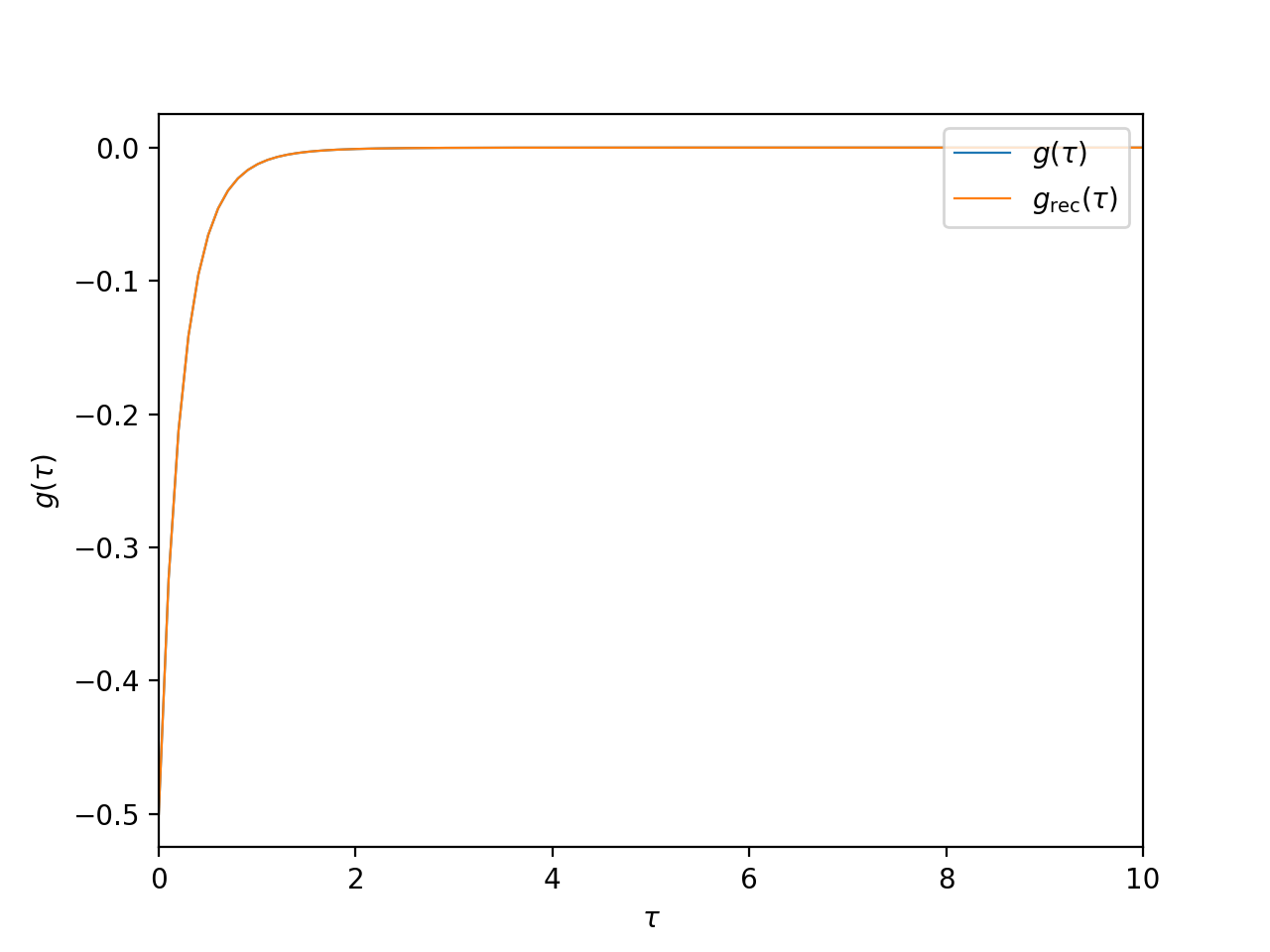
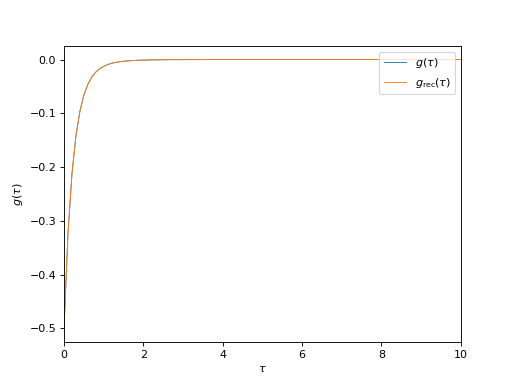
Plot input and reconstructed imaginary-time correlators

from pytriqs.gf.local import *
from pytriqs.archive import HDFArchive
from matplotlib import pyplot as plt
from pytriqs.plot.mpl_interface import oplot

# Read data from archive
ar = HDFArchive('results.h5', 'r')

# Plot input and reconstructed correlator
oplot(ar['g_tau'],     mode='R', linewidth=0.8, label="$g(\\tau)$")
oplot(ar['g_rec_tau'], mode='R', linewidth=0.8, label="$g_\mathrm{rec}(\\tau)$")

plt.xlim((0, 10))
plt.ylabel("$g(\\tau)$")
plt.legend(loc="upper right")

(Source code, png, hires.png, pdf)

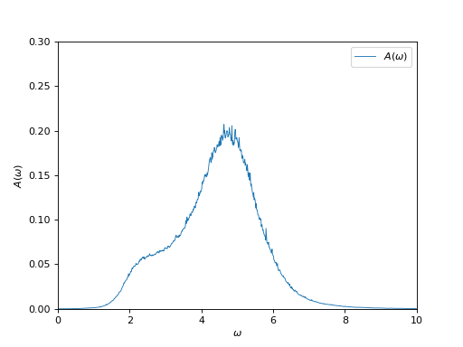
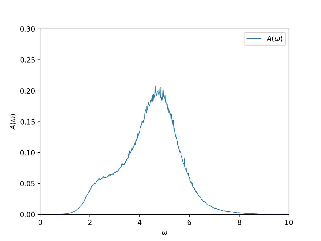
Plot the spectral function

from pytriqs.gf.local import *
from pytriqs.archive import HDFArchive
from matplotlib import pyplot as plt
from pytriqs.plot.mpl_interface import oplot

# Read data from archive
ar = HDFArchive('results.h5', 'r')

# Plot the spectral function
oplot(ar['g_w'], mode='S', linewidth=0.8, label="$A(\\omega)$")

plt.xlim((0,10.0))
plt.ylim((0,0.3))
plt.ylabel("$A(\\omega)$")
plt.legend(loc = "upper right")

(Source code, png, hires.png, pdf)