Example: Fermionic Green’s function or self-energy

Observable kind: FermionGf.

Note

With FermionGf one can also continue a self-energy function as long as it does not contain a static Hartree-Fock contribution (decays to 0 at \(\omega\to\infty\)). In this case norms must be precomputed separately as first spectral moments of the self-energy.

For derivation of spectral moments see, for instance,

"Interpolating self-energy of the infinite-dimensional Hubbard model:
Modifying the iterative perturbation theory"
M. Potthoff, T. Wegner, and W. Nolting, Phys. Rev. B 55, 16132 (1997)

Run analytical continuation

# Import some TRIQS modules and NumPy
from pytriqs.gf.local import *
from pytriqs.archive import HDFArchive
import pytriqs.utility.mpi as mpi
import numpy

# Import main SOM class
from pytriqs.applications.analytical_continuation.som import Som

n_tau = 500                 # Number of tau-slices for the input GF

n_w = 801                   # Number of energy slices for the solution
energy_window = (-4.0,4.0)  # Energy window to search the solution in


# Parameters for Som.run()
run_params = {'energy_window' : energy_window}
# Verbosity level
run_params['verbosity'] = 3
# Number of particular solutions to accumulate
run_params['l'] = 2000
# Number of global updates
run_params['f'] = 100
# Number of local updates per global update
run_params['t'] = 50
# Accumulate histogram of the objective function values
run_params['make_histograms'] = True

# Read G(\tau) from archive
# Could be G(i\omega_n) or G_l as well.
g_tau = HDFArchive('example.h5', 'r')['g_tau']
# g_tau stored in example.h5 has a dense mesh with 10001 slices

# Prepare input data: reduce the number of \tau-slices from 10001 to n_tau
g_input = rebinning_tau(g_tau, n_tau)

# Set the weight function S to a constant (all points of g_tau are equally important)
S = g_input.copy()
S.data[:] = 1.0

# Construct a SOM object
#
# Expected norms of spectral functions can be passed to the constructor as
# norms = numpy.array([norm_1, norm_2, ..., norm_N]), where N is the matrix
# dimension of g_input (only diagonal elements will be continued). All norms
# are set to 1.0 by default.
cont = Som(g_input, S, kind = "FermionGf", norms = numpy.array([1.0, 1.0]))

# Run!
# Takes 5-10 minutes on 16 cores ...
cont.run(**run_params)

# Evaluate the solution on an energy mesh
# NB: we can use *any* energy window at this point, not necessarily that from run_params
g_w = GfReFreq(window = (-5.0,5.0), n_points = n_w, indices = [0,1])
g_w << cont

# G(\tau) reconstructed from the solution
g_rec_tau = g_input.copy()
g_rec_tau << cont

# On master node, save results to an archive
if mpi.is_master_node():
    with HDFArchive("results.h5",'w') as ar:
        ar['g_tau'] = g_tau
        ar['g_rec_tau'] = g_rec_tau
        ar['g_w'] = g_w
        ar['histograms'] = cont.histograms

Download input file example.h5.

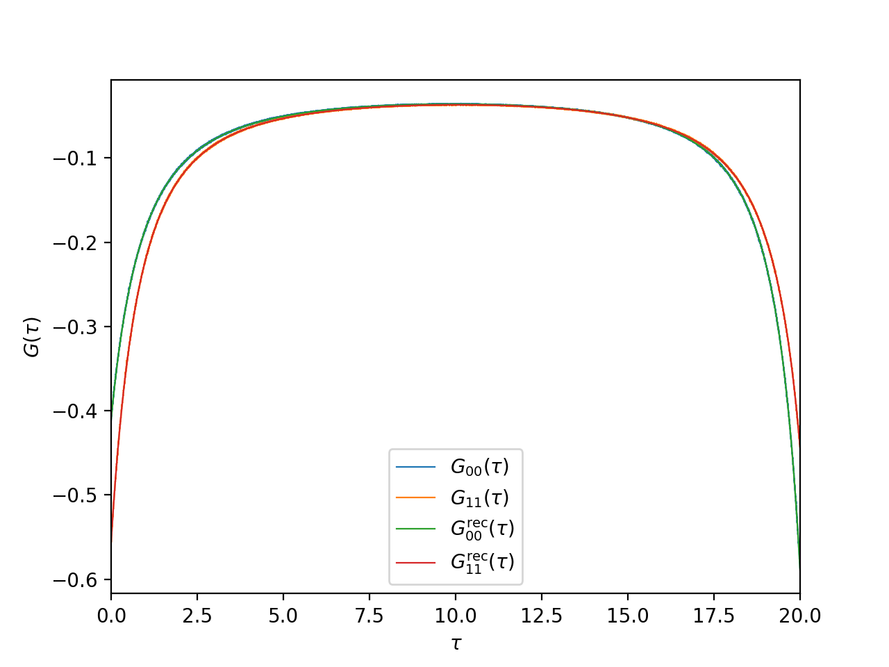
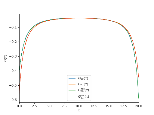
Plot input and reconstructed imaginary-time GF’s

from pytriqs.gf.local import *
from pytriqs.archive import HDFArchive
from matplotlib import pyplot as plt
from pytriqs.plot.mpl_interface import oplot

# Read data from archive
ar = HDFArchive('results.h5', 'r')

# Plot input and reconstructed G(\tau)
oplot(ar['g_tau'][0,0],     mode='R', linewidth=0.8, label="$G_{00}(\\tau)$")
oplot(ar['g_tau'][1,1],     mode='R', linewidth=0.8, label="$G_{11}(\\tau)$")
oplot(ar['g_rec_tau'][0,0], mode='R', linewidth=0.8, label="$G_{00}^\mathrm{rec}(\\tau)$")
oplot(ar['g_rec_tau'][1,1], mode='R', linewidth=0.8, label="$G_{11}^\mathrm{rec}(\\tau)$")

plt.xlim((0, 20))
plt.ylabel("$G(\\tau)$")
plt.legend(loc="lower center")

(Source code, png, hires.png, pdf)

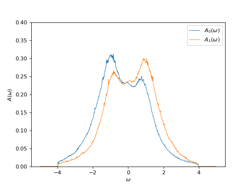
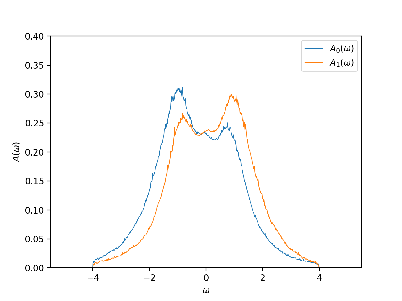
Plot the spectral function

from pytriqs.gf.local import *
from pytriqs.archive import HDFArchive
from matplotlib import pyplot as plt
from pytriqs.plot.mpl_interface import oplot

# Read data from archive
ar = HDFArchive('results.h5', 'r')

# Plot the spectral functions
oplot(ar['g_w'][0,0], mode='S', linewidth=0.8, label="$A_0(\\omega)$")
oplot(ar['g_w'][1,1], mode='S', linewidth=0.8, label="$A_1(\\omega)$")

plt.ylim((0,0.4))
plt.ylabel("$A(\\omega)$")

(Source code, png, hires.png, pdf)