Example: Correlator of boson-like operators

Observable kind: BosonCorr.

A general correlation function of boson-like operators \(\hat O\) and \(\hat O^\dagger\) is defined as

\[\chi(\tau) = \langle\mathbb{T}_\tau \hat O(\tau) \hat O^\dagger(0)\rangle.\]

\(\chi(\tau)\) is subject to an additional periodicity condition

\[\chi(\tau+\beta) = \chi(\tau).\]

Examples of such correlators are the transverse magnetic susceptibility \(\langle\mathbb{T}_\tau \hat S_+(\tau) \hat S_-(0)\rangle\) and the Green’s function of bosons \(\langle\mathbb{T}_\tau \hat b(\tau) \hat b^\dagger(0)\rangle\).

The auxiliary spectral function \(A(\epsilon) = \Im\chi(\epsilon)/\epsilon\) is non-negative but not necessarily symmetric.

Warning

When \(\hat O = \hat O^\dagger\) (for instance, in case of charge or longitudinal magnetic susceptibility), it is strongly recommended to use BosonAutoCorr observable kind instead.

Run analytical continuation

# Import some TRIQS modules and NumPy
from pytriqs.gf.local import *
from pytriqs.archive import HDFArchive
import pytriqs.utility.mpi as mpi
import numpy

# Import main SOM class
from pytriqs.applications.analytical_continuation.som import Som

n_w = 1001                    # Number of energy slices for the solution
energy_window = (-5.0,5.0)    # Energy window to search the solution in


# Parameters for Som.run()
run_params = {'energy_window' : energy_window}
# Verbosity level
run_params['verbosity'] = 3
# Number of particular solutions to accumulate
run_params['l'] = 10000
# Number of global updates
run_params['f'] = 100
# Number of local updates per global update
run_params['t'] = 50
# Accumulate histogram of the objective function values
run_params['make_histograms'] = True

# Read \chi(i\omega_n) from archive
# Could be \chi(\tau) or \chi_l as well.
chi_iw = HDFArchive('example.h5', 'r')['chi_iw']

# Set the weight function S to a constant (all points of chi_iw are equally important)
S = chi_iw.copy()
S.data[:] = 1.0

# Construct a SOM object
#
# Norms of spectral functions are known to be 3.0 for both diagonal components of \chi.
# It is possible to estimate the norms as \pi\chi(i\omega_0) (estimate affected by noise)
cont = Som(chi_iw, S, kind = "BosonCorr", norms = numpy.array([3.0, 3.0]))

# Run!
# Takes 10-15 minutes on 16 cores ...
cont.run(**run_params)

# Evaluate the solution on an energy mesh
# NB: we can use *any* energy window at this point, not necessarily that from run_params
chi_w = GfReFreq(window = (-5.0,5.0), n_points = n_w, indices = [0,1])
chi_w << cont

# \chi(i\omega_n) reconstructed from the solution
chi_rec_iw = chi_iw.copy()
chi_rec_iw << cont

# On master node, save results to an archive
if mpi.is_master_node():
    with HDFArchive("results.h5",'w') as ar:
        ar['chi_iw'] = chi_iw
        ar['chi_rec_iw'] = chi_rec_iw
        ar['chi_w'] = chi_w
        ar['histograms'] = cont.histograms

Download input file example.h5.

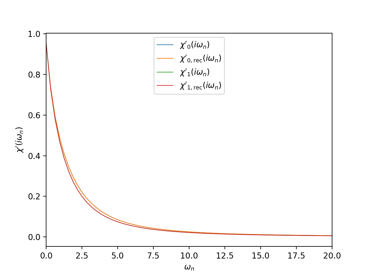
Plot input and reconstructed correlators at Matsubara frequencies

from pytriqs.gf.local import *
from pytriqs.archive import HDFArchive
from matplotlib import pyplot as plt
from pytriqs.plot.mpl_interface import oplot

# Read data from archive
ar = HDFArchive('results.h5', 'r')

# Plot input and reconstructed \chi(i\omega_n), real parts
oplot(ar['chi_iw'][0,0],     mode='R', linewidth=0.8, label="$\chi'_0(i\\omega_n)$")
oplot(ar['chi_rec_iw'][0,0], mode='R', linewidth=0.8, label="$\chi'_\mathrm{0,rec}(i\\omega_n)$")
oplot(ar['chi_iw'][1,1],     mode='R', linewidth=0.8, label="$\chi'_1(i\\omega_n)$")
oplot(ar['chi_rec_iw'][1,1], mode='R', linewidth=0.8, label="$\chi'_\mathrm{1,rec}(i\\omega_n)$")

plt.xlim((0, 20))
plt.ylabel("$\chi'(i\\omega_n)$")
plt.legend(loc="upper center")
plt.show()

(Source code, png, hires.png, pdf)

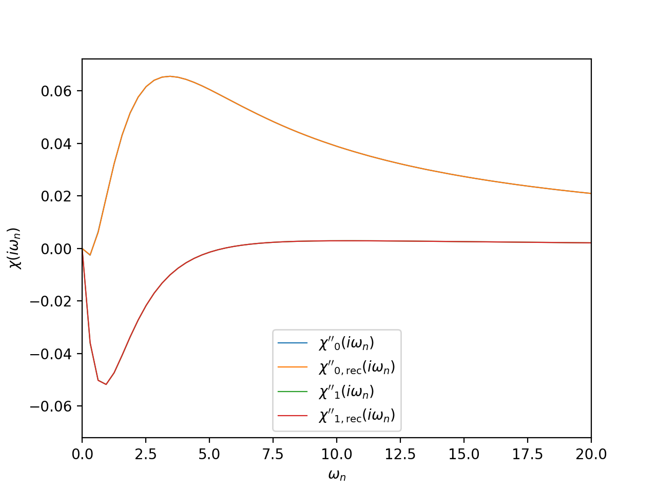
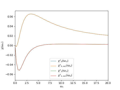
# Plot input and reconstructed \chi(i\omega_n), imaginary parts
oplot(ar['chi_iw'][0,0],     mode='I', linewidth=0.8, label="$\chi''_0(i\\omega_n)$")
oplot(ar['chi_rec_iw'][0,0], mode='I', linewidth=0.8, label="$\chi''_\mathrm{0,rec}(i\\omega_n)$")
oplot(ar['chi_iw'][1,1],     mode='I', linewidth=0.8, label="$\chi''_1(i\\omega_n)$")
oplot(ar['chi_rec_iw'][1,1], mode='I', linewidth=0.8, label="$\chi''_\mathrm{1,rec}(i\\omega_n)$")

plt.xlim((0, 20))
plt.ylabel("$\chi(i\\omega_n)$")
plt.legend(loc="lower center")

(png, hires.png, pdf)

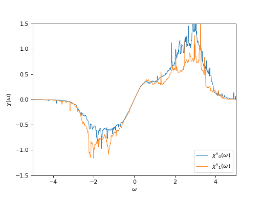
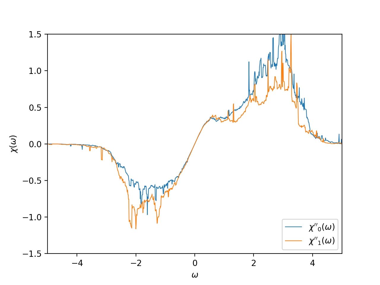
Plot the correlator on the real frequency axis

from pytriqs.gf.local import *
from pytriqs.archive import HDFArchive
from matplotlib import pyplot as plt
from pytriqs.plot.mpl_interface import oplot

# Read data from archive
ar = HDFArchive('results.h5', 'r')

# Plot imaginary part of the susceptibility on the real axis
oplot(ar['chi_w'][0,0], mode='I', linewidth=0.8, label="$\chi''_0(\\omega)$")
oplot(ar['chi_w'][1,1], mode='I', linewidth=0.8, label="$\chi''_1(\\omega)$")

plt.xlim((-5.0,5.0))
plt.ylim((-1.5,1.5))
plt.ylabel("$\chi(\\omega)$")
plt.legend(loc = "lower right")

(Source code, png, hires.png, pdf)